I have written a coupe of Matlab scripts to implement tube plotting and exporting the tubes for modeling and raytracing programs. The package is free for anybody to use.
Download tubeplot package. Contains tubeplot.m, frenet.m, frame.m and saveobjtube.m
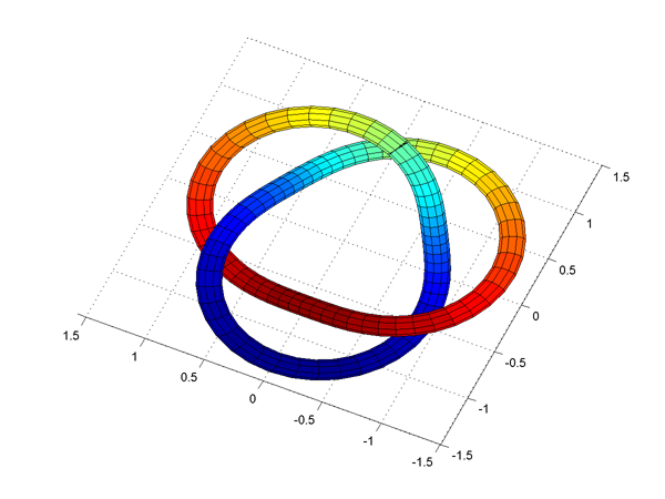
The basic script is tubeplot.m. It plots 3D curves as thickened tubes:
t=0:(2*pi/100):(2*pi);
x=cos(t*2).*(2+sin(t*3)*.3);
y=sin(t*2).*(2+sin(t*3)*.3);
z=cos(t*3)*.3;
tubeplot(x,y,z,0.14*sin(t*5)+.29,sin(t),10)
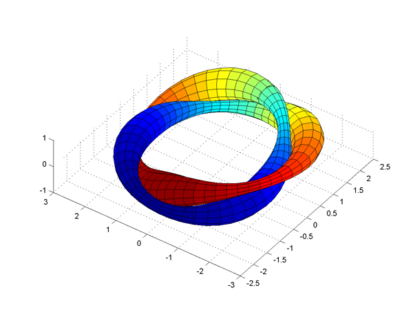
Here the tube has a variable radius and coloring, and 10 subdivisions around its circumference.
This can produce some drawbacks when the curve has an inflection point:
x=cos(t*2).*(1+sin(t*3)*.3);
y=sin(t*2).*(1+sin(t*3)*.3);
z=cos(t*3)*.3;
tubeplot(x,y,z,0.1,sin(t),10)
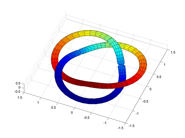
Here the mesh twists 180 degrees as the normal flips side. Increasing the resolution does not help much. One way around this is to calculate the frame not using the second derivative of the curve (which becomes parallel to the tangent at such points) but using an arbitrary vector that is never parallel to the tangent (see frame.m):
tubeplot(x,y,z,0.1,sin(t),10,[0 0 1])
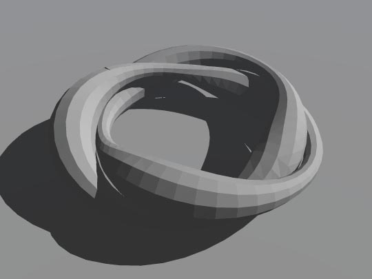
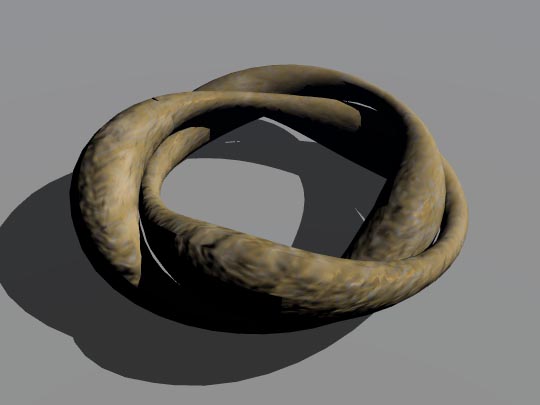
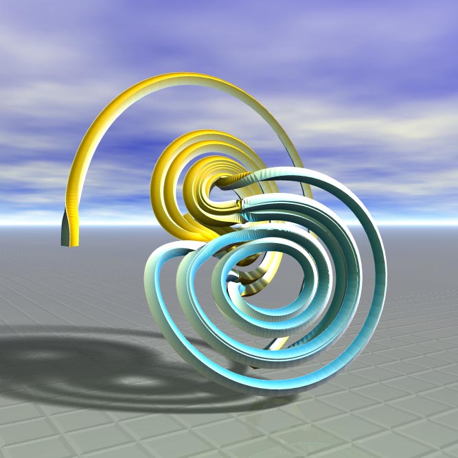
Once loaded it can be smoothed and textured:
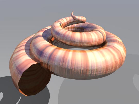
t=0:.1:20;
x=t.*sin(t);
y=t.*cos(t);
z=t;
r=t/3;
saveobjtube('shell.obj',x',y',z',r',1,10)
The texture is by default mapped as an unit square wrapped around each tube.
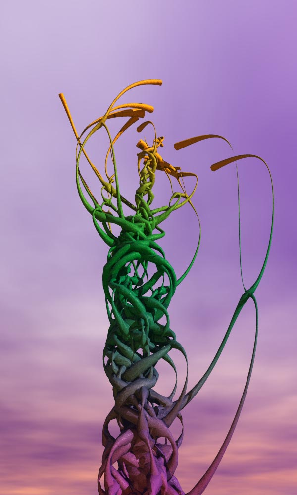
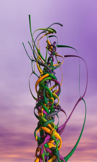
This image shows the spacetime paths of particles moving in an 1/(r^2 + epsilon) gravity field with some friction slowing them down. Time is running downwards. Starting from the top the particles slow down, form pairs and clusters that merge into the central chaotic trunk. The velocity is used to set the tube radius, while color is based on time (orange = at the start, violet = near end).
Here the second parametrisation option was used, making textures different on different tubes. This generally helps distinguishing them, although not much in this case.
Here a low resolution tube is useful to show how the Frenet frame is carried around the attractor. By coloring it so that different sides of the frame have different colors and not smoothing it in Bryce it is possible to see a rather nontrivial property of the attractor. The dynamics does not mix the direction of the Frenet frame, so the two lobes have differently colored sides. There are no yellow streaks on the blue side, and vice versa. So regardless of the chaotic switching between the lobes the sense of "right" and "up" relative to the trajectory is not changed. In an attractor with a Möbius band geometry they would switch each orbit.